Machine learning potentials

Looking up values in literature is one way to make a Pourbaix diagram. But what if we’re interested in a novel material that has not been tested experimentally yet?

In materials science, the goal is often to find new materials with desirable properties. For example: an oxygen evolution catalyst that doesn’t corrode at low pH, a battery electrolyte with high ion conductivity, or a battery electrode that doesn’t swell during charging. Testing those materials in a lab is time-consuming. The field of computational materials science develops methods to screen new materials with calculations. The best candidate materials are tested in the lab.

In this part you will learn about modern methods that are used for screening materials.

Electronic structure methods

The most important contribution to the internal energy \(U\) of a material is the energy of the electrons interacting with the nuclei. You can think of this energy as the “chemical binding energy”. Electrons are best described by quantum mechanics. The field of electronic structure theory develops methods to calculate the behavior of electrons as accurately as possible. Examples of these methods are Hartree-Fock theory and density functional theory (DFT).

The calculations are very costly: they can take minutes to hours on a supercomputer. The figure below shows that a large part of supercomputing facilities is used for such electronic structure calculations. They also require expertise for choosing certain approximation parameters.

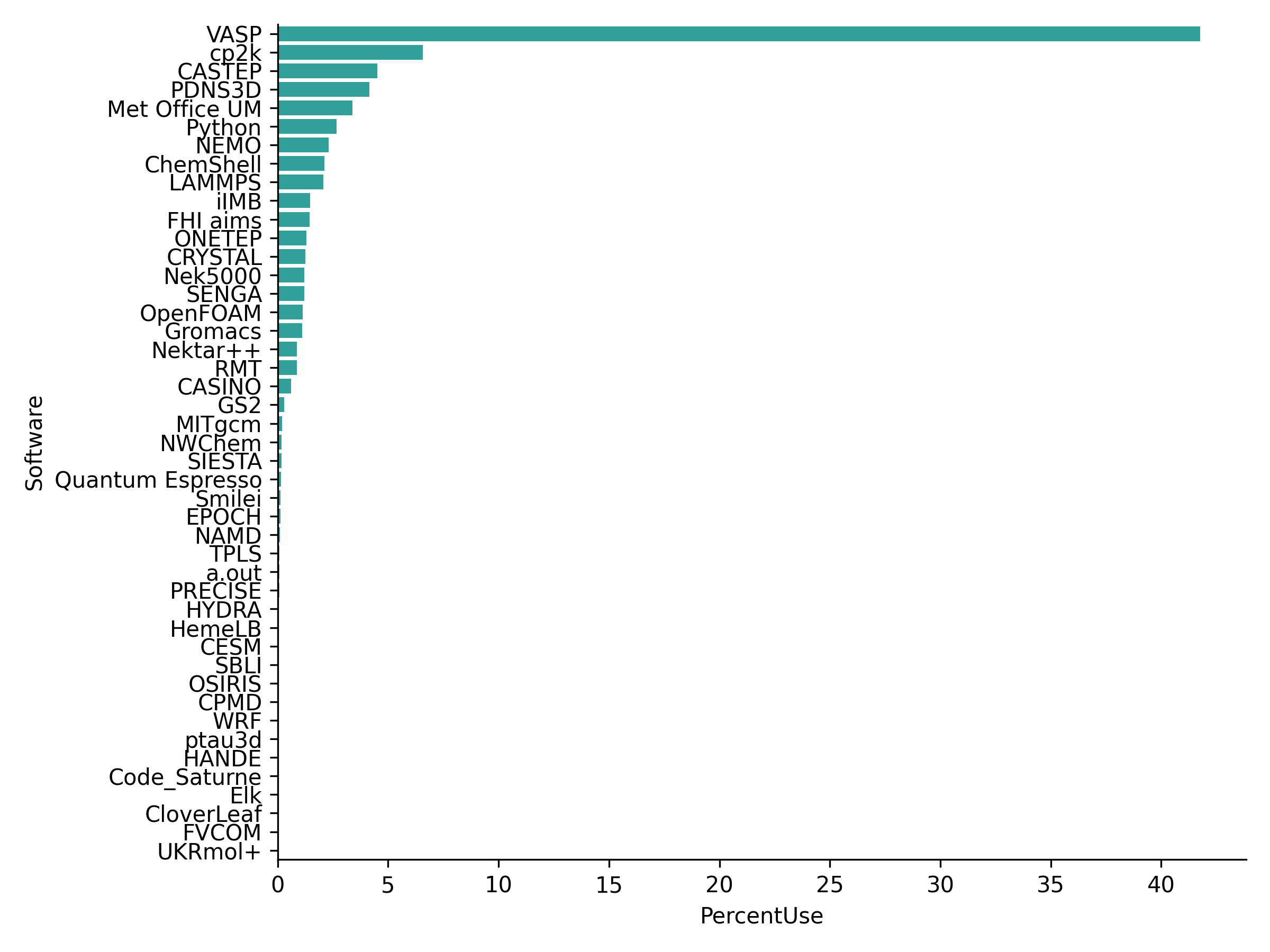
Fig. 3 Usage of the British high-performance computing facility for various tasks in January 2022. VASP, CP2K and CASTEP are examples of quantum chemistry softwares. Source: archer2.

If you want (optional), you can read more about electronic structure methods on the page Extra: Quantum chemistry from last year’s LO1.

Machine learning

Often, we don’t even need all the electronic structure information. Given a certain atomistic structure we just want to know the energy, and sometimes the forces on the nuclei. In recent years, machine learning models have been developed to predict energies and forces for atomistic structures [4]. A model that predicts the energy depending on the distance between particles is often called a ‘potential’ (like the Lennard-Jones potential). A machine learning model that predicts energies and forces on atoms is called a machine learning interatomic potential (MLIP).

In general, a machine learning model represents a function \(f\). The function \(f\) is learned from a ‘training set’ containing data points \(x_i\) with a label \(y_i\). In atomistic machine learning, \(x_i\) represents the structure of a material (like the coordinates of all the atoms and their chemical elements), and \(y_i\) is the energy. Given a point \(x_i\), the machine learning model predicts a label \(\hat{y}_i=f(x_i)\).

To train the model, a loss function

\[\mathcal{L} = \sum_i (\hat{y}_i-y_i)^2\]

is minimized (for a more in-depth explanation, see 3blue1brown on YouTube). In words: the training procedure finds a function \(f\) so that all \(\hat{y}_i\) are as close as possible to the corresponding \(y_i\).

The function \(f\) representing the potential can be quite complicated. Over the past decade, a lot of research has gone into designing functions that describe atomistic structures efficiently. Symmetry is an important aspect: if you rotate a molecule in vacuum, its energy does not change. Many modern models are designed so that rotation of the structure does not change the energy [5].

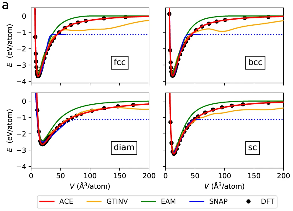
Fig. 4 Comparison of various machine learning potentials with the training data from DFT, from [6]. The plots above show potential energy vs. separation between atoms in a crystal lattice.

Question

Consider the figure above. Compare to a Morse potential. Does the potential look like what you would expect?

In addition to designing a model, we need a training set. A training set is usually made by calculating the energy \(y_i\) of atomic structures \(x_i\) with DFT. This has two important consequences:

• The accuracy of the model depends on how accurate the energy calculated with DFT is. So it’s still important to understand what approximations were made in the DFT calculations used to construct the training set.

• The model can predict the energy of new structures \(x_i\) that are similar to the training data. If you train a model only on water molecules, it probably cannot predict the energy of a metal. But it might also fail to predict the energy of a molecule if it has a weird structure (very short/large interatomic distance) that does not appear in the training set.

So: it is important to understand the training set!

In the beginning, machine learning models were trained on specialized datasets. If you were interested in copper, you would train the model on a bunch of copper metal structures. But over the last two years, models have been trained on huge datasets containing many different materials and molecules. Although their predictions are not as accurate as quantum chemistry calculations, they provide a pretty good guess and are very fast. These big models are called foundational models.

In the rest of this lab we will use machine learning interatomic potentials to calculate the energy of metal and metal oxide structures. Specifically, we’ll use foundational models with the MACE architecture [7, 8]. To install MACE, open your terminal/Anaconda prompt and type pip install mace-torch (as usual, feel free to ask for help). You’ll also need ase, which should be installed automatically when installing mace-torch, but if not you can type pip install ase.

Note

Machine learning in chemistry is a hot topic: Microsoft, Meta, the Chinese company DP Tech and the start-ups Radical AI, Cusp AI and Orbital Materials are all working on machine learning potentials. Cusp AI is co-founded by Max Welling, a Dutch professor at UvA, and Radical AI is co-founded by Gerbrand Ceder from the paper on Pourbaix diagrams [3] that a lot of the theory we use in this practical is based on.

In case you’re still confused: the Microsoft keynote gives a nice introduction to machine learning in chemistry (they talk about potentials, but also generative models).

Oxygen molecule

Let’s see how this all works in practice. First, we use ASE to define the structure of an oxygen molecule. Note: viewer='x3d' is for IPython notebooks, which were used to generate this web page. If you run a .py file, you should just use view(material).

from ase.build import molecule
from ase.visualize import view
atoms = molecule('O2')
view(atoms, viewer='x3d')

(This is the kind of atomic structure that would be an \(x_i\) for a machine learning model.) Now, let’s load a MACE model and predict the energy. Download the MACE-MATPES-r2SCAN-0 model from github.com/ACEsuit/mace-foundations, and place it in the same folder as your Python script. On the bottom of the download page, you can find what publication you need to cite in your report!

from mace.calculators import mace_mp

calc = mace_mp(model="MACE-matpes-r2scan-omat-ft.model", default_dtype="float64")
atoms.calc = calc
atoms.get_potential_energy()

C:\Users\kamlbtde\AppData\Local\miniconda3\envs\mace\Lib\site-packages\e3nn\o3\_wigner.py:10: UserWarning: Environment variable TORCH_FORCE_NO_WEIGHTS_ONLY_LOAD detected, since the`weights_only` argument was not explicitly passed to `torch.load`, forcing weights_only=False.
  _Jd, _W3j_flat, _W3j_indices = torch.load(os.path.join(os.path.dirname(__file__), 'constants.pt'))

cuequivariance or cuequivariance_torch is not available. Cuequivariance acceleration will be disabled.

Using float64 for MACECalculator, which is slower but more accurate. Recommended for geometry optimization.

C:\Users\kamlbtde\AppData\Local\miniconda3\envs\mace\Lib\site-packages\mace\calculators\mace.py:143: UserWarning: Environment variable TORCH_FORCE_NO_WEIGHTS_ONLY_LOAD detected, since the`weights_only` argument was not explicitly passed to `torch.load`, forcing weights_only=False.
  torch.load(f=model_path, map_location=device)

Using head default out of ['default']

-11.746797198194443

The energy you get out is the electronic energy, we’ll call it \(E^\mathrm{DFT}\).

The MACE-MATPES-r2SCAN-0 model is trained with r2SCAN-DFT data, which should be more accurate than the “standard” model you get when you use model="medium", which is trained with PBE-DFT. Try model="medium" and run the code again to see the difference in energy.

We can also optimize the bond length with a BFGS optimizer:

from ase.optimize import BFGS

optimizer = BFGS(atoms)
optimizer.run(fmax=0.001)  # maximum force in eV/Angstrom

      Step     Time          Energy          fmax
BFGS:    0 14:58:21      -11.746797        1.905323

BFGS:    1 14:58:23      -11.742271        2.348481

BFGS:    2 14:58:24      -11.773124        0.204156

BFGS:    3 14:58:24      -11.773393        0.019630

BFGS:    4 14:58:24      -11.773396        0.000189

True

The optimizer prints the different steps in which it changes the bond length to minimize the forces on the atoms until they are below fmax (at room temperature, the oxygen molecule will be in a state where the forces are close to zero). As you can see, the energy difference is quite small, but it could make a difference in the end, so geometry optimization is recommended.

Finally, we can write the atoms to an XYZ file:

from ase.io import write

write("oxygen_molecule.xyz", atoms)

Look into the xyz file and try to understand the structure of the file.

Materials

For metals and metal oxides, we can find molecular structures online. For example, the Crystallography Open Database contains many experimental structures. Search for a structure relevant to your Pourbaix diagram by providing the different elements (like Fe, O) and the number of distinct elements (min. 2, max. 2 for example). In the results, click on ‘CIF’ to download the CIF structure file. You can read it in ASE:

from ase.io import read

material = read("structures/Li2O.cif")
view(material, viewer='x3d')

C:\Users\kamlbtde\AppData\Local\miniconda3\envs\mace\Lib\site-packages\ase\io\cif.py:410: UserWarning: crystal system 'cubic' is not interpreted for space group Spacegroup(225, setting=1). This may result in wrong setting!
  warnings.warn(

You can again find \(E^\mathrm{DFT}\):

calc = mace_mp(model="MACE-matpes-r2scan-omat-ft.model", default_dtype="float64")
material.calc = calc
material.get_potential_energy()

C:\Users\kamlbtde\AppData\Local\miniconda3\envs\mace\Lib\site-packages\mace\calculators\mace.py:143: UserWarning: Environment variable TORCH_FORCE_NO_WEIGHTS_ONLY_LOAD detected, since the`weights_only` argument was not explicitly passed to `torch.load`, forcing weights_only=False.
  torch.load(f=model_path, map_location=device)

Using float64 for MACECalculator, which is slower but more accurate. Recommended for geometry optimization.

Using head default out of ['default']

-67.11994532427966

You can also optimize the unit cell size and geometry:

from ase.filters import UnitCellFilter

material.calc = calc
ucf = UnitCellFilter(material)
opt = BFGS(ucf)
opt.run(fmax=0.001)

      Step     Time          Energy          fmax
BFGS:    0 14:58:26      -67.119945        0.131128

BFGS:    1 14:58:28      -67.120677        0.129183

BFGS:    2 14:58:29      -67.144967        0.000812

True

Task

Download structures for all the materials you can find in the experimental Pourbaix diagram. Calculate the energy with the r2SCAN MACE model. Save the energies for the oxygen molecule and the other structures.

You can leave out the ions – calculating the energy of an ion in water is difficult. If optimizing the structures is too much effort you can also skip that.

Tip: to be consistent with literature and the equations we used to calculate \(\Delta \mu\), calculate the energy per formula unit. A structure might contain 12 nickel atoms and 16 oxygen atoms, but we want the energy for \(\mathrm{Ni_2 O_3}\).